7. absolute value linear inequalities (2)
절대값일차부등식
absolute value linear inequalities
"그래프를 활용하니까 절대값부등식도
이해가 너무 쉽고 잘 외워져요"
" function graph makes it easier
to solve absolute value inequalities "
기본형이 아닌 절대값
부등식은, 절대값 안의
값이 양 (+) 인지 음
(–) 인지에 따라, 경우를
나누어 계산하는 것이
원칙입니다.
따라서, 반드시 구간을 나누어
생각해야 하고, 각각의
구간별 풀이는 교집합 (∩) 과 합집합 (∪) 을 논리적으로 정확하게 적용해야 하는 사고력 훈련의 대표적인 유형입니다.
물론, 이 경우에도
그래프를 이용해서 쉽게
문제를 해결할 수
있습니다. 특히, 이
방법은 이차 또는
고차부등식에서 그대로 활용할
수 있는
개념이므로, 해결과정을 확실하게
이해해 두어야 합니다.
이
단원 역시 매우
중요한 내용이므로, 반드시
기본개념과 응용력을 철저히
익혀두시기 바랍니다.
♧ ♧ ♧ ♧ ♧ ♧
스마트폰에서 수학 수식을 보시려면, 왼쪽 버튼을 누른 후
[데스크톱 보기] 를 설정하세요.
Please select [desktop view] on the mobile
to read math equations
♧ ♧ ♧ ♧ ♧ ♧
절대값이
여러 개가 포함되거나
숫자가 아닌 식이
포함된 절대값부등식은, 앞에서
배운 기본형과는 달리, 절대값 안의 값의
부호가 바뀌는 값을
기준으로, 구간들을 나누어서
푸는 것이 원칙입니다.
Supposing the
inequality has more than one absolute bar or it has equations instead of
number, it is a standard solution to divide into intervals where the values
within the absolute bar become positive (+) or negative (–).
우선, 보기 문제를
풀어 볼까요?
Let's start with a worked example.
아래의 절대값 부등식을 풀어라.
Find the solution set of following inequality.
| x –
2 | < \(\frac{1}{2}\)x + 1
(1) 우변이 숫자만 있는
기본형이 아니고, 식이
들어 있으니까, 절대값
안의 부호가 바뀌는 2 를 기준으로, 두 가지의 경우로 나누어 풀어야
합니다.
This inequality
has an equation on the right hand side instead of a number and therefore, we
have to divide into two intervals where the value within the bar become positive
(+) or negative (–).
(A) x < 2 일 때
|
(B) x ≥ 2 일 때
|
– x
+ 2 < \(\frac{1}{2}\)x + 1
∴ x
>\(\frac{2}{3}\)
|
x – 2 < \(\frac{1}{2}\)x + 1
∴ x
< 6
|
(2) 앞의 [절대값 일차방정식] 단원에서 배웠던, 논리 다이어그램으로 보면, (A ∩ P) ∪ (B ∩ Q) 의 개념입니다. 다시 복습이 필요한 분은 아래의 링크를 참고하세요.
We've already
learned to use logic diagram (A ∩ P) ∪ (B ∩ Q) in [ linear absolute value equation ] before.
If you want to review again, please refer to the above link.
( \(\frac{2}{3}\) < x < 2) ∪ (2 ≤ x < 6)
∴ \(\frac{2}{3}\) < x < 6
이번에는 똑같은 문제를 그래프를 이용해서 풀어 보도록 할까요?
This time,
let's a try different approach of using function graphs in a
coordinate plane.
(1) 부등식 | x –
2 | < \(\frac{1}{2}\)x + 1 의 좌변과 우변을 각각의 함수로 간주해서 아래와 같이 좌표평면에 그래프로 나타냅니다.
Consider each
side of inequality as a function and draw its graph on the coordinate plane
as shown below.
y = f (x)
= | x – 2 | vs. y
= g (x) = \(\frac{1}{2}\)x + 1

(2) 위의 그래프를 보고, 파란색의 직선인 y = f (x) = | x –
2 | 가 빨간색의 직선인 y = g
(x) = \(\frac{1}{2}\)x + 1 보다 작다고 했으니까, 위 그래프에 있는 노란색의 영역을 찾아 냅니다.
As shown above, the
solution set will be yellow shaded region where the blue v-shape line y =
f (x) = | x – 2 | is below the red horizontal line y =
g
(x)
= \(\frac{1}{2}\)x + 1.
(3) x 에 관한 부등식을 푸는 것이니까, 부등식의 영역도 x 값을 기준으로 좌표평면에 표시하도록 합니다. x = \(\frac{2}{3}\) 와 x = 6 인 양 끝 경계선은 포함되지 않는다는 점에 주의하세요.
We're solving x-term inequalities and therefore, the
yellow solution set region should be expressed only in terms of x. Be careful that boundary lines x = \(\frac{2}{3}\) and x = 6 will not be included.
∴ \(\frac{2}{3}\) < x < 6
이번에는 절대값이 두 개인 문제를 풀어
보도록 할까요?
This time, let's try to solve the inequality that has
two absolute bars.
아래의 절대값 부등식을 풀어라.
Find the solution set of following inequality.
| x +
2 | – | x – 1 | ≥ 0
(1) 절대값이 두 개가 들어 있으니까, 절대값 안의 부호가
바뀌는 – 2 와 1 을
기준으로, 3 가지의 경우로 나누어 풀어야 하겠지요?
This inequality
has two absolute bars and therefore we have to divide into three intervals at –
2 and 1 where the value within the bar becomes positive (+) or negative (–).
(A) x < –
2일 때
|
(B) – 2 ≤ x < 1 일 때
|
(C) x ≥ 1 일 때
|
– x
– 2 + x – 1 ≥ 0
이는 모순
∴
Ø
|
x + 2 + x
– 1 ≥ 0
∴ x
≥
|
x + 2 – x
+1 ≥ 0
항상 참
∴ x 는
모든 실수
|
(2) 앞의 [절대값 일차방정식] 단원에서 배웠던, 논리 다이어그램으로 보면, (A∩P) ∪ (B∩Q) ∪ (C∩R) 의 개념입니다.
We've already
learned to use logic diagram (A∩P) ∪ (B∩Q) ∪ (C∩R) in [linear absolute value equation].
( Ø ) ∪ ( \( - \frac{1}{2}\) ≤ x < 1 ) ∪ ( 1 ≤ x )
∴ x ≥ \( - \frac{1}{2}\)
이번에는 똑같은 문제를 그래프를 이용해서 풀어 보도록 할까요?
This time,
let's a try to solve differently by using function graphs in a
coordinate plane.
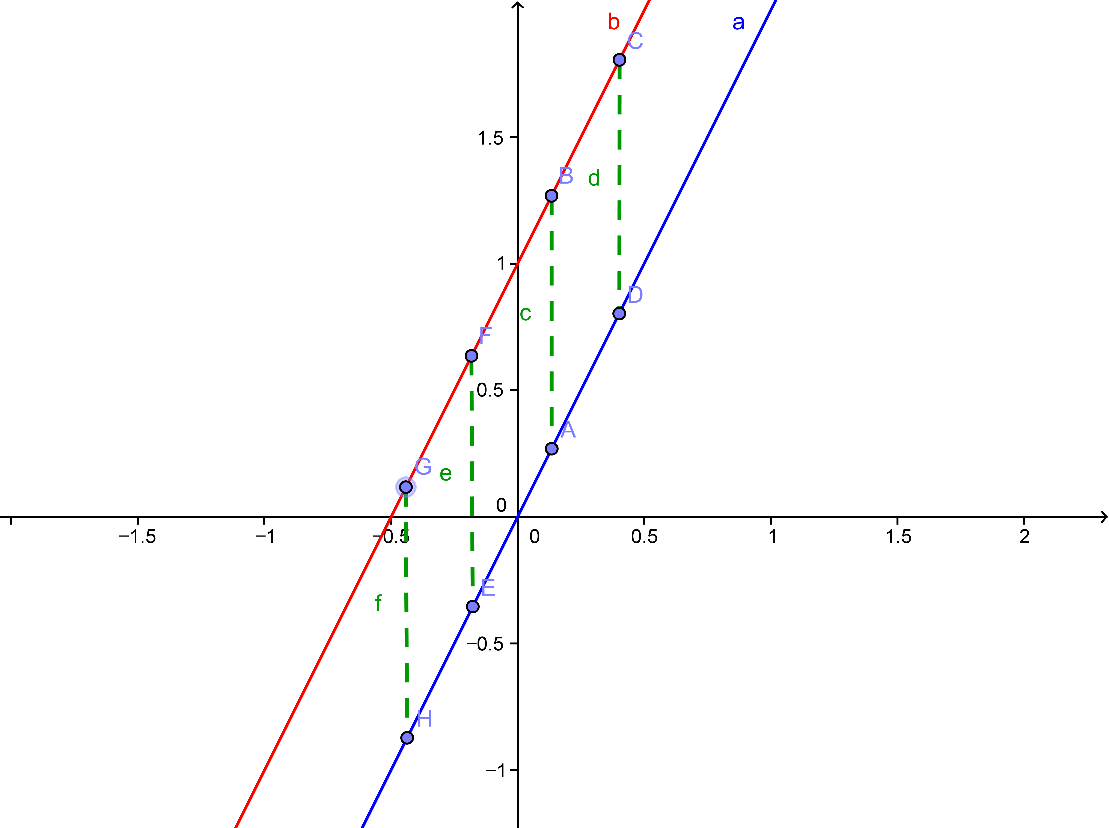
(1) 그리기 쉽도록, 부등식을 | x + 2 | ≥ | x – 1 | 로 바꾼
다음, 좌변과 우변을 각각의 함수로 간주해서 아래와 같이 좌표평면에 그래프로 나타냅니다.
In order to compare
more clearly, rearrange the inequality and consider each side of inequality as
a function and sketch its graph on the coordinate plane as shown below.
y = f (x) = | x + 2 | vs. y = g (x)
= | x – 1 |

(2) 위의 그래프를 보고, 파란색의 꺽은선인 y = f (x) = | x +
2 | 가 빨간색의 꺽은선인 y = g
(x) = |
x – 1 | 보다 크거나 같다고
했으니까, 위 그림에
있는 노란색의 영역을
찾아 냅니다.
As shown above, the
solution set will be yellow shaded region where the blue v-shape line y =
f (x) = | x + 2 | is below the red v-shape line y =
g
(x)
= | x – 1 |.
(3) x 에 관한 부등식을 푸는 것이니까, 부등식의 영역도 x 값을 기준으로 좌표평면에 표시하도록 합니다. x = \( - \frac{1}{2}\) 인 경계선이
포함된다는 점에 주의하세요.
We're solving x-term inequalities and therefore, the
yellow solution set region should be expressed only in terms of x. Be careful that boundary line x =
will
be included.
∴ x ≥
그래프를 그려내는 실력을 어느 정도 갖추게 되면,
주어진 방정식이나 부등식을 자기가 편리한 방법으로 고친 다음, 쉽고 간단하게 그래프를 이용해서
문제를 해결해 낼 수 있습니다.
If you are
accustomed drawing function graphs, then you can rearrange the equations or
inequalities to be suitable for easier sketch or comparison in solving them.
이 그래프를 이용하는
방법은 향후 고등수학이나 상위수학의 이차 또는 고차부등식등에서 그대로 활용할 수 있는 개념이므로, 해결과정을
확실하게 이해해 두고, 방정식이나 부등식을 풀 때나 혹은 다른 방법으로 검산할 때 자주 활용해 봄으로써, 응용력을 키워 나가기 바랍니다.
This graph
method is a very powerful tool to solve polynomial equations or inequalities in
higher level math. I hope you to understand the underlying core concept and try
to make the best use of it.
Comments
Post a Comment